The case against the fluffy metrics: Rate of force development (part 3)

Introduction
In the last article we went a little deeper into how the methods we use to calculate rate of force development (RFD) from isometric mid-thigh pull (IMTP) force-time data can influence it. And, quite frankly, it can get very messy very quickly. The key points to take from it though is that, where possible, you should try to take real ownership of your data; try to find out and understand how your force plate system calculates RFD (well, all metrics really) and any limitations there may be to that method, especially when it comes to comparing your data to others whose data may have been calculated from a completely different method. Now, enough on the IMTP because I can almost hear you shouting:

          'what about the countermovement jump, can we get useful RFD data from them?'

Now, obviously here at Hawkin Dynamics we're in the business of making force plate based athlete assessment accessible to all. We think we've done a pretty good job of this too. Of course, we would say that, but bear with me. In this article I'll not only take you through the way we calculate countermovement vertical jump (CMJ) RFD, but, to reinforce the importance of using robust and repeatable methods, what happens when different methods are used to calculate CMJ RFD.

CMJ RFD - the Hawkin Dynamics way

It shouldn't come as a surprise to read that we've tried to use what we think is the simplest and most robust, repeatable method to calculate CMJ RFD. This is really important to us because, as you'll see as through this article, even more different methods have been used to calculate CMJ RFD than have been used to calculate IMTP RFD.

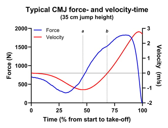
Figure 1. A typical CMJ force- and velocity-time curve. The blue curve is the force-time curve, while the red curve is the velocity-time curve. Time has been normalised relative to the duration of the period between the start of the jump and take-off. The horizontal grey line represents zero velocity. Vertical line a and b represent the start of the braking (positive acceleration down sub-phase) and propulsion (up phase).

Now, consider Figure 1 that shows a typical CMJ force- and velocity-time curve, and we can use the velocity-time curve to help us identify key locations. The horizontal, dark grey line represents zero velocity. Remember then that everything below this means that the jumper's center of mass is moving downwards, while everything above this means that the jumper's center of mass is moving upwards. Therefore, vertical line a represents the beginning of what is frequently referred to as the 'braking' phase, while vertical line b represents the beginning of what is frequently referred to as the 'propulsion' or 'up' phase. Essentially, our method identifies the force at these points, calculates the change in force by subtracting the lowest velocity force from the lowest displacement force and then divides this by the time between these two points.

In the Figure 1 example we get the following information:

• Force at lowest velocity (line a) = 702 N
• Force at lowest displacement (line b) = 1523 N
• Therefore, the change in force = 821 N
• This occurs over 0.165 s
• Therefore, 821 / 0.165 = 4975 N/s (newtons per second) or 68 N/kg/s (normalized relative to body mass)

Simple! But what does it mean? Well, like I suggested in the last blog, there are no magic metrics. We need to understand what they represent, and perhaps more importantly how and why they change for them to be useful. With this in mind, let's consider Figure 2 and 3, which show the force-time curves from a 20 cm and a 47 cm CMJ, respectively. You'll see that I've marked the beginning of the braking and propulsion phases again, but what else to you notice? Yep, although their respective braking phase duration is within 10 milliseconds of one another (0.160 and 0.170 s respectively), the 47 cm jumper applied 1428 N or 15 N/kg to brake their downward movement while the 20 cm jumper applied 994 N or 11 N/kg. This means that the 20 cm jumper's RFD was 6218 N/s or 71 N/kg/s, while the 47 cm jumper's RFD was 8400 N/s or 89 N/kg/s. So, more braking force in a similar braking duration, which equals a steeper force-time curve. Does this explain the 27 cm difference in jump height? I'd say yes, absolutely. However, remember that this doesn't mean that we should only consider this metric, it's part of a bigger picture with regards to these jumper's driver and strategy metrics. For example, we could also calculate how quickly these jumpers performed their down phase. The lowest velocity for these jumps was The 20 cm jumper's lowest velocity was -0.91 meters per second (m/s), while the 47 cm jumper's lowest velocity was -1.69 m/s. Because we know (from the impulse-momentum theorem) that impulse is proportional to the change in velocity multiplying these velocities by the jumper's body mass will give us the impulse they applied during the braking phase. 

• 20 cm jumper braking impulse = -79.18 Ns (newton seconds)
• 47 cm jumper braking impulse = -159 Ns (newton seconds) 

Why might this be useful? In my humble opinion I think it's useful because, from a mechanical perspective, it is directly related to jump performance.  We can't necessarily say the same about RFD. However, that isn't the biggest potential problem. Oh no, thinking back to the last article, I'm now going to take you through some of methodological factors that can influence CMJ RFD so strap in.

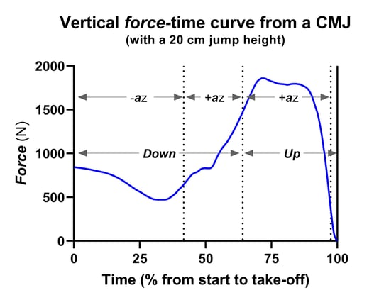Figure 2. Force-time curves from a 20 cm CMJ. As per Figure 1, time has been normalised relative to the duration of the period between the start of the jump and take-off.

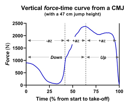Figure 3. Force-time curves from a 47 cm CMJ. As per Figure 1, time has been normalised relative to the duration of the period between the start of the jump and take-off.

Now, if you were paying me for my opinion on whether you should use CMJ RFD or not, I would say 'it depends'. This might seem like a cop-out, but it really isn't. Remember, you can, in theory at least, use any metric just as long as you honestly say that you understand how you got it, what it represents, and what its limitations are. With that in mind, I would much rather recommend braking impulse in addition to the force and time components it's derived from. I won't unfollow you on social media though if you choose RFD.

The effect of method on CMJ RFD

So, how does method affect CMJ RFD? For this comparison I'm going to back to the 35 cm CMJ featured in Figure 1. We know that to jump 35 cm they applied a braking phase RFD of 4975 N/s (or 68 N/kg/s when normalized relative to body mass). Let's consider the most common methods that have been used in the literature to calculate CMJ RFD and compare them to the Hawkin Dynamics method:

• Hawkin Dynamics method =

• Instantaneous RFD calculated by differentiating (dividing changes in force by time) force data on a sample-by-sample basis when force was filtered (or not) using the following methods:
  • Unfiltered force data
  • Force data filtered using a Butterworth filter with a cut-off frequency of 50 Hz (a pretty common and not too harsh an approach. More of the original data is retained. This is what HD does)
  • Force data filtered using a Butterworth filter with a cut-off frequency of 10 Hz (what should be a less common approach - a very harsh approach because a lot of the original data is removed)
  • Force data filtered using a moving average filter where data are averaged over 10 data points (not too harsh an approach. Most of the original data is retained)
  • Force data filtered using a moving average filter where data are averaged over 40 data points (a very harsh method because a lot of the original data is removed. Data may also move to the right)

What does our comparison show us?

Figure 4 shows the five different RFD-time curves from our 35 cm jumper's force data. Figure 5 and 6 zoom in on the different method's RFD during the down and up phases respectively. As with the IMTP data that we discussed in previous blog posts, the first thing you'll probably notice is that there is a lot of difference between RFD calculated from the different methods. Thankfully the general shape of the curves is very similar across the different methods. However, the magnitudes aren't. And this is where the problems start for the study of RFD in dynamic tasks like the CMJ. What you should also notice is that, perhaps counter-intuitively, CMJ RFD is negative during the propulsion phase (lowest displacement to take-off).

Take a closer look at Figure 5. After an initial decrease, RFD starts to increase as we arrive at the lowest countermovement force (the first dotted vertical line). John Harry and colleagues have recently proposed a new down sub-phase that they refer to as yielding. They've shown that negative lower-body joint power during this sub-phase, and the RFD data in Figure 5 seems to support this. What does this mean? Well, it appears that, perhaps passively, we begin to put the brakes on to slow downward displacement earlier than many of us have thought for a while. Very interesting. Exciting even. But we need more research into this before we get too excited. It could hold some exciting potential with regards to athlete assessment and training prescription. Keep an eye on John Harry's work.  

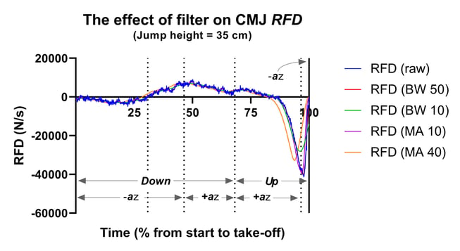Figure 4. The effect of method on CMJ RFD.

RFD = rate force development; BW 50 = force data treated with a Butterworth filter with a cut-off frequency of 50 Hz (a pretty common and not too harsh an approach. More of the original data is retained. This is what HD does); BW 10 = force data treated with a Butterworth filter with a cut-off frequency of 10 Hz (a harsh approach because a lot of the original data is removed); MA 10 = force data treated with a moving average filter where force data is averaged over 10 samples (most of the original data is retained); MA 40 = force data treated with a moving average filter where force data are averaged over 40 samples (a lot of the original data is removed).

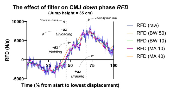Figure 5. The effect of method on down phase CMJ RFD.

RFD = rate force development; BW 50 = force data treated with a Butterworth filter with a cut-off frequency of 50 Hz (a pretty common and not too harsh an approach. More of the original data is retained. This is what HD does); BW 10 = force data treated with a Butterworth filter with a cut-off frequency of 10 Hz (a harsh approach because a lot of the original data is removed); MA 10 = force data treated with a moving average filter where force data is averaged over 10 samples (most of the original data is retained); MA 40 = force data treated with a moving average filter where force data are averaged over 40 samples (a lot of the original data is removed).

The second dotted vertical line in Figure 5 marks the lowest countermovement velocity, the start of what we often refer to as the braking phase. We can see that while RFD is still positive, it is decreasing and it continues to do so until we reach the down-up phase transition. This is also perhaps the first opportunity to see the effect that our different methods have on the magnitude of RFD. First, look how jagged RFD from the raw force-time data is (the blue line). These data are noisy! We can also see that the red and purple curves (BW 50 and MA 10 respectively, the relatively gentle filtering methods that retain most of the original data) closely match the pattern of our raw RFD, but the worst of the noise has been removed. Now compare that with the green and orange curves (BW 10 and MA 40 respectively, more harsh filtering methods that remove a lot of the original data).      

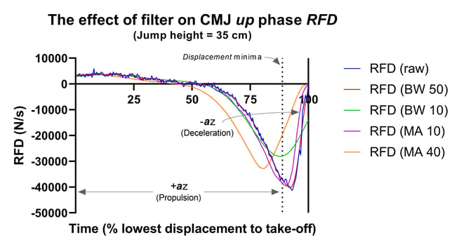Figure 6. The effect of method on up phase CMJ RFD.

RFD = rate force development; BW 50 = force data treated with a Butterworth filter with a cut-off frequency of 50 Hz (a pretty common and not too harsh an approach. More of the original data is retained. This is what HD does); BW 10 = force data treated with a Butterworth filter with a cut-off frequency of 10 Hz (a harsh approach because a lot of the original data is removed); MA 10 = force data treated with a moving average filter where force data is averaged over 10 samples (most of the original data is retained); MA 40 = force data treated with a moving average filter where force data are averaged over 40 samples (a lot of the original data is removed).

Now, let's focus on the up phase. To reiterate, RFD is mostly negative, and however potentially counter-intuitive, this should not come as too much of a surprise once we've reminded ourselves of the nature of the CMJ. We often use this test to gauge ones elastic capacity or stiffness. That's right, how effectively the jumper can use their stretch-shortening cycle (SSC). There are a number of theories to explain the performance improvement to be gained from the SSC. I think that Cormie et al. (2010) provide the best summary in the work they published in 2010. Basically however, either energy generated or contraction potential developed during the stretch of the countermovement enhances up phase performance. And this is why up phase RFD tends to be mostly negatively. We're unloading rather than actively developing force. And if you're scratching your head and asking yourself whether I really know what I'm talking about, don't worry, if you haven't come across this before it can really mess with your head. Trust me though, I'm not making this up. And this is why CMJ peak force tends to occur around the down-up phase transition.

It's time to consider our last figure, Figure 7. Apart from using a flamboyant colour scheme, you can really see the effect that method has on RFD magnitude here. The largest effect can be found in the peak (from the braking phase) RFD (green bars), with a range of 197, 164 N/s!! Yes, that's over 8000% more than the Hawkin Dynamics method. It really does pay to understand where your data comes from. It's not all lost though. Look at the pink and orange bars. They're relatively consistent across the different methods that we've considered in this blog. In fact, the method-based variance tends to lurk at around 3%. Not too bad. Of course, the braking mean RFD is considerably larger than the HD RFD (around 213%), but the difference across the different force data filtering methods remains fairly consistent (around 3%). And, finally, we have the olive green bars to remind us that propulsion phase RFD is both negative and more variable (around 18%).   

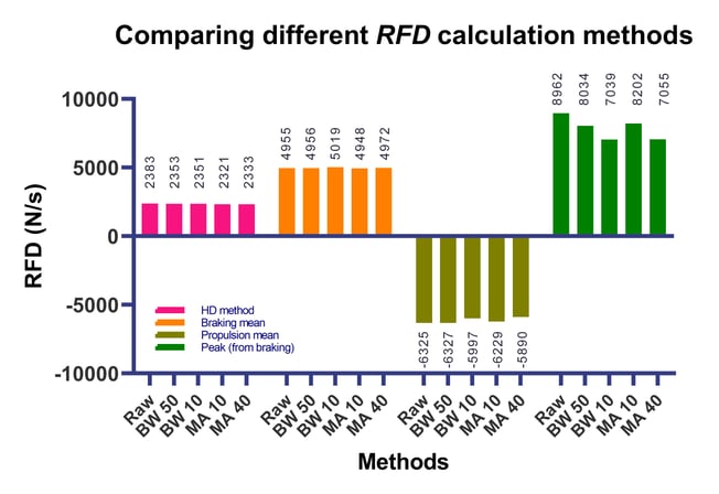
Figure 7. The effect of method and phase on the magnitude of CMJ RFD .  

Conclusion

Okay, so was my doom and gloom cursing of the RFD in the ODSF metrics blog a little premature. Unkind maybe? My bottom line is that I stand by that article. Not so much because of my academic ivory tower ego, but because while RFD, like power, can be useful, can yield important information there are far more useful metrics. Again, at the risk of belabouring the point, while RFD and power can be related to performance, they do not dictate it. Certainly not from a mechanical perspective. And I'd go as far as saying that while they can be useful, they have the potential to cause confusion in the wrong hands. So, the key take-home points, as always, are as follows:

• You can use any metric you want to use. However, you must understand its strengths and limitations (including calculation method limitations)
• Try to develop as robust a rationale as you possibly can for using any metrics you think will help you tell your jump performance story
• Avoid using a single metric to try and tell what can be a relatively complicated story (yes, a task as seemingly simple as jumping can be complex)
• Again for those in the back of the room: Please, I implore you, understand how your metrics have been calculated
• And remember, if a company won't tell you how they calculate their metrics I'd strongly suggest finding another company (there should be no secrets, Newton gave us the blueprint for this stuff several hundred years ago!)
• The same goes for any analysis software that's been passed around - understand the calculations before you decide by any of the metrics it calculates (especially if your athlete's performance and job might depend on it)

Now, finally, as sad as this might sound, I love this stuff. I love studying it and writing about it. So if you have any questions or if you have any areas that you'd like us to discuss in the Hawkin Dynamics 'Talkin' Force' webinars or you'd like me to write about (complete with awesome graphs) then please do get in touch.