-2.png?width=156&height=60&name=Hawkin%20Logo%20(2)-2.png)
.png?width=780&height=439&name=ForceDisplacement_JLake72023%20(2).png)
Image 1: Overlayed force-displacement (position) loops normalized to time.
Introduction
If you are interested in how vertical jump force-time data can be presented you will notice that there are a myriad of ways to do this. This is cool. After all, a sensible amount of variety can help those interested contextualize what they're looking at. However, if you're anything like me then it can sometimes feel like there is too much going on. Do you stick with what you know or invest the time and energy needed to understand the utility of what the new (or just different) method can give us? For clarity, we're going to be focusing on data from the countermovement vertical jump (CMJ).
Force-displacement and Force-velocity Loops
One example of this is the recent increase in the use of the so-called force-displacement and force-velocity loops. Before we move on, I think a quick definition and illustration are needed to make sure that we're all on the same page with these. It should be noted that the force-displacement loop can also be referred to as the force-position loop, or "work loop". But don't worry, they're all the same thing.
To create a force-displacement loop we do the following:
1. Identify the start of the jump
2. Identify the takeoff
3. Crop both force and displacement relative to these points
4. Plot our new force data against our new displacement data
To create a force-velocity loop we do the following
1. Repeat steps 1 & 2
2. Crop the velocity data relative to the start and takeoff
3. Plot our new force data against our new velocity data
Force-displacement and force-velocity loops from an exemplar CMJ with a 39 cm jump height, and the force data these came from are presented in Figures 1, 2, and 3. How do we interpret them though?
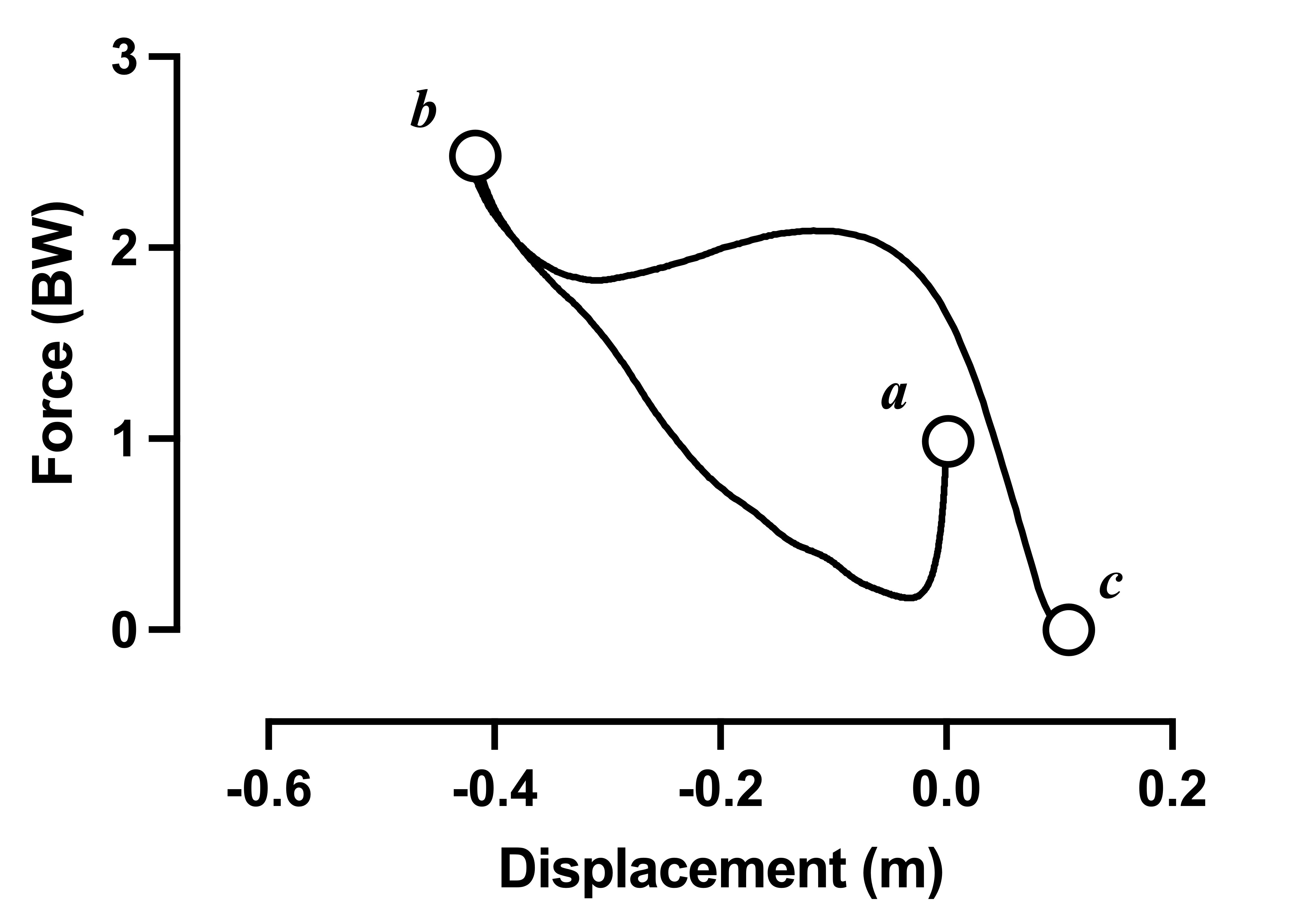
Figure 1: Force-displacement loop with force normalized to body weight.
Well first, let's orientate ourselves. If we think about this logically, what will force be at the start and end (takeoff) of the CMJ? At the beginning, it will be around the jumper's body weight (i.e. system weight). I've normalized force data by dividing it by the jumper's body weight (recorded in newtons). Therefore, the start force should be one body weight. The force at the end of the jump will be around 0 N (because this is the point the jumper leaves the ground). If we look at both Figures 1 and 2 we can see that this is the case.
Another way to conceptualize this is to look at the displacement. At the jump-start, the position should be zero (because they're standing still), and we shouldn't be surprised to see that, as the jumper rises onto their toes immediately before they leave the ground, their position is greater than zero. Remember that when we derive displacement and velocity from force plate force data it reflects the jumper's center of mass (the point around which all mass is distributed).
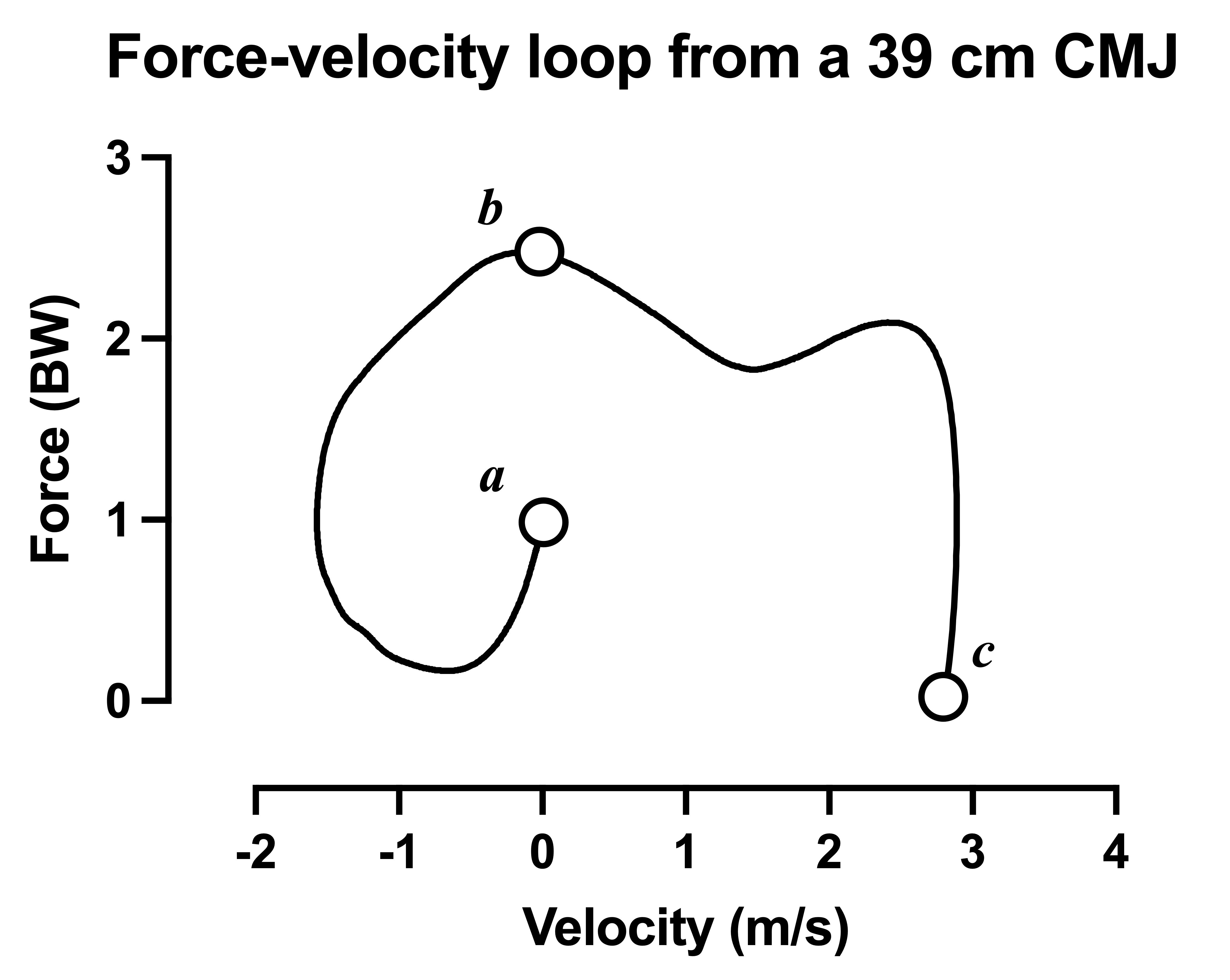
Figure 2: Force-velocity loop with force normalized to body weight.
A more extreme example can be seen if we consider the velocity in the force-velocity loop. As with displacement, we will again begin at zero velocity. As the jumper approaches takeoff though you'll notice a far more dramatic increase in velocity (relative to the force-displacement loop), that continues to a peak before tapering off (slightly) immediately before takeoff. This is the point of peak velocity.
The force-time curve has been annotated below in Figure 3. Briefly, annotations represent the following:
a. The start of the jump
b. Peak negative force
c. Peak negative velocity
d. Peak force
e. Peak negative position
f. Peak velocity
g. Takeoff
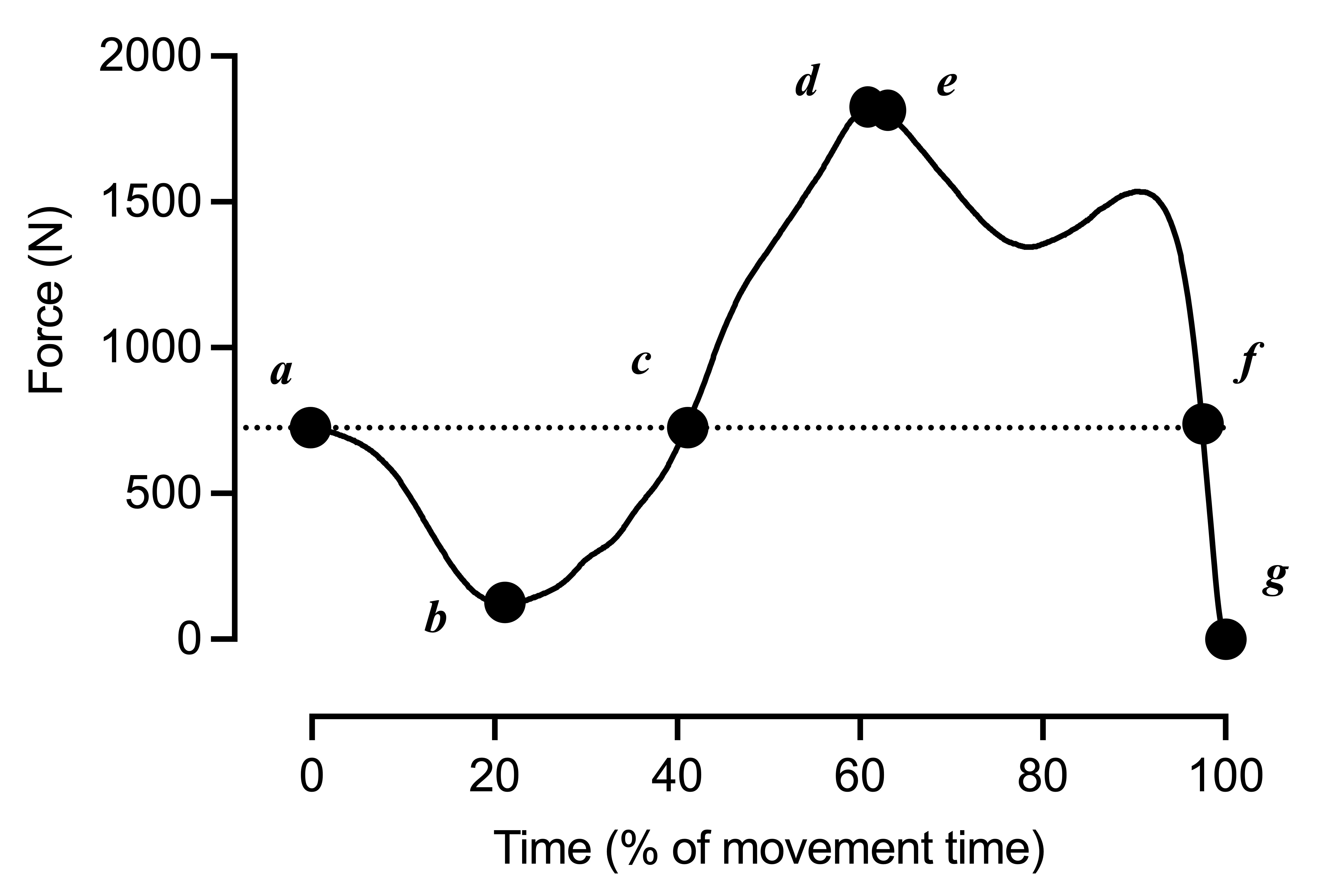
Figure 3: Annotated force-time curve from the same CMJ as in Figure 2 and Figure 1.
Historical Context
I was trying to think back to when I first came across these loops. My initial thought was in some of the excellent work presented by Prue Cormie. Now, I know (and I'm pretty sure they would totally acknowledge this) that they weren't the first to do this, but they made excellent use of them to demonstrate the effect that different training strategies could have on human neuromuscular capacity.
Force-velocity plots (or curves) have been and continue to be used. In addition to the work by Prue Cormie (see above), excellent examples of these can be traced back to the work of Hill (1938) and Kaneko et al. (1983) (and no doubt countless others). These shouldn't, of course, be confused with the work driven by Morin and Samozino, who have plotted discrete force and velocity data points from progressively loaded vertical jumps to assess what they've referred to as force-velocity imbalances. A critique of this is far beyond the scope of this blog but may interest some of you.
Comparing jumpers of different abilities
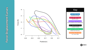
So, how can we use force-displacement and force-velocity loops? To illustrate this, Drake (Berberet) randomly selected data from the CMJ performance of three random jumpers (Image 1 above has six randomly selected jumpers). Their respective force-time curves are presented below in Figure 4. Again, you'll see that I've normalized the force by dividing it by each jumper's body weight. Additionally, I've normalized it relative to the movement time of each jump (from the jump start to takeoff). Finally, you can see that I've classified each jumper using a red, amber, and green 'traffic light' coding system. This is based on the key performance metrics of jump height, movement time, and reactive strength index modified (mRSI) with our 'red' jumper demonstrating the lowest performance level in this case, the 'green' jumper the highest level, and the 'amber' jumper performing somewhere in the middle. Their data are presented in Table 1.
Table 1. Some of the main CMJ performance metrics from our three different jumpers.
| Red | Amber | Green | |
| Mass (kg) | 68.713 | 83.245 | 85.817 |
| Jump height (m) | 0.269 | 0.462 | 0.654 |
| Movement time (s) | 0.728 | 0.697 | 0.637 |
| RSImod | 0.369 | 0.667 | 1.026 |
| Unweighting time (% of movement time) | 42% | 47% | 56% |
| Braking time (% of movement time) | 20% | 19% | 15% |
| Propulsive time (% of movement time) | 38% | 35% | 28% |
| Peak force (N) | 1647.00 | 2341.25 | 3226.00 |
| Peak force (BW) | 23.97 | 28.13 | 37.59 |
| Peak negative velocity (m/s) | -1.2065 | -1.508 | -1.556 |
| Braking net force (N) | 552.920 | 941.671 | 1338.643 |
| Braking impulse (Ns) | 81.832 | 123.359 | 131.187 |
| Propulsive net force (N) | 577.259 | 1050.464 | 1714.646 |
| Propulsive impulse (Ns) | 158.746 | 253.162 | 308.636 |
(A) Their force-time curves
Depending on how far you are into your CMJ force data education, you'll likely notice a few differences between the three jumpers as soon as you set eyes on Figure 4. For the sake of consistency though, the first step in our analysis of these three jumpers should be to consider the pattern (or shape) and magnitude (or how much) force that underpinned each jumper's performance. We can get an idea of how quickly force was applied by looking at how steep any of the slopes are. However, of course, the time element has been blurred somewhat by my normalizing data to movement time (see Table 1). It shouldn't be a surprise to see that the 'red' jumper applies the least force relative to body weight and appears to apply it less quickly than the 'amber' and 'green' jumper. In fact, the 'green' jumper is clearly way ahead.
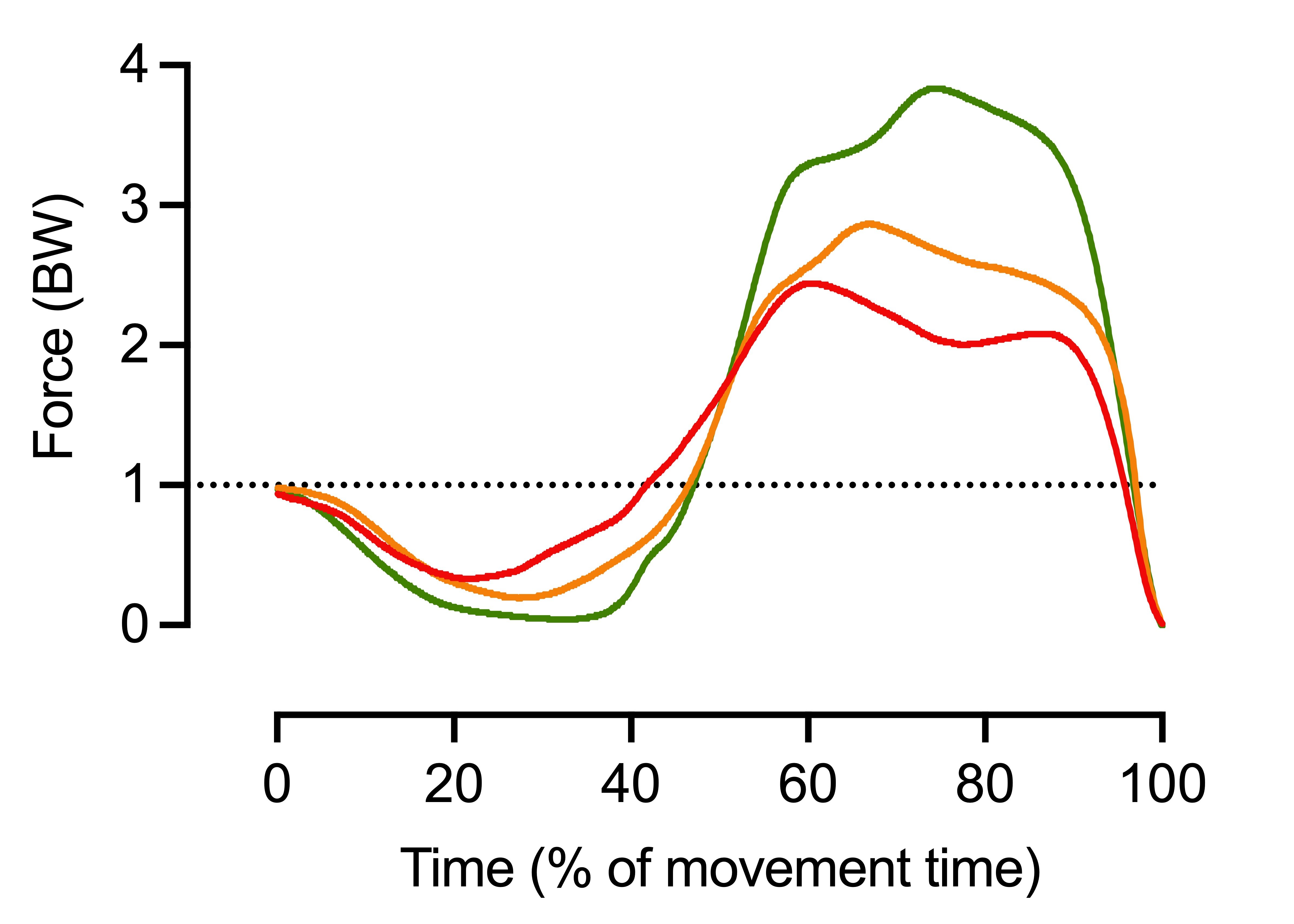
Figure 4: Three colored force-time curves showing differences in jump strategies.
(B) Their force-displacement loops
The force-displacement loops from each jumper have been overlayed in Figure 5. Naturally, they reflect much of what we saw in Figure 4. Each jumper, from 'red' to 'green', applies progressively more force during the propulsive phase of the jump. However, if we consider the loops between points 'a' and 'b' we'll see that the same pattern is repeated in the way each jumper 'unloads' during the countermovement phase. One thing to note is that while the 'green' jumper performs the most shallow 'squat', the depth of the 'red' jumper's countermovement displacement is less than that of the 'amber' jumper. This should serve as an important reminder of why we should try to avoid focusing on one (or a few) key metrics because, and this should be obvious, we get less of a story of the jumper's capacity. From points 'b' to 'c' we can see that our 'green' jumper applies theirs propulsive force more quickly than the 'amber' jumper who applies their propulsive force more quickly than the 'red' jumper. I think you'll agree that this is reasonably straightforward. And it might help you get a clearer understanding of the strategy element that we often talk about in CMJ force data analysis. For me though, the force-velocity loop can be even more informative because it takes some of the guesswork of the time element out of it because we have a visual record of how quickly the jumper is moving between the start and takeoff.
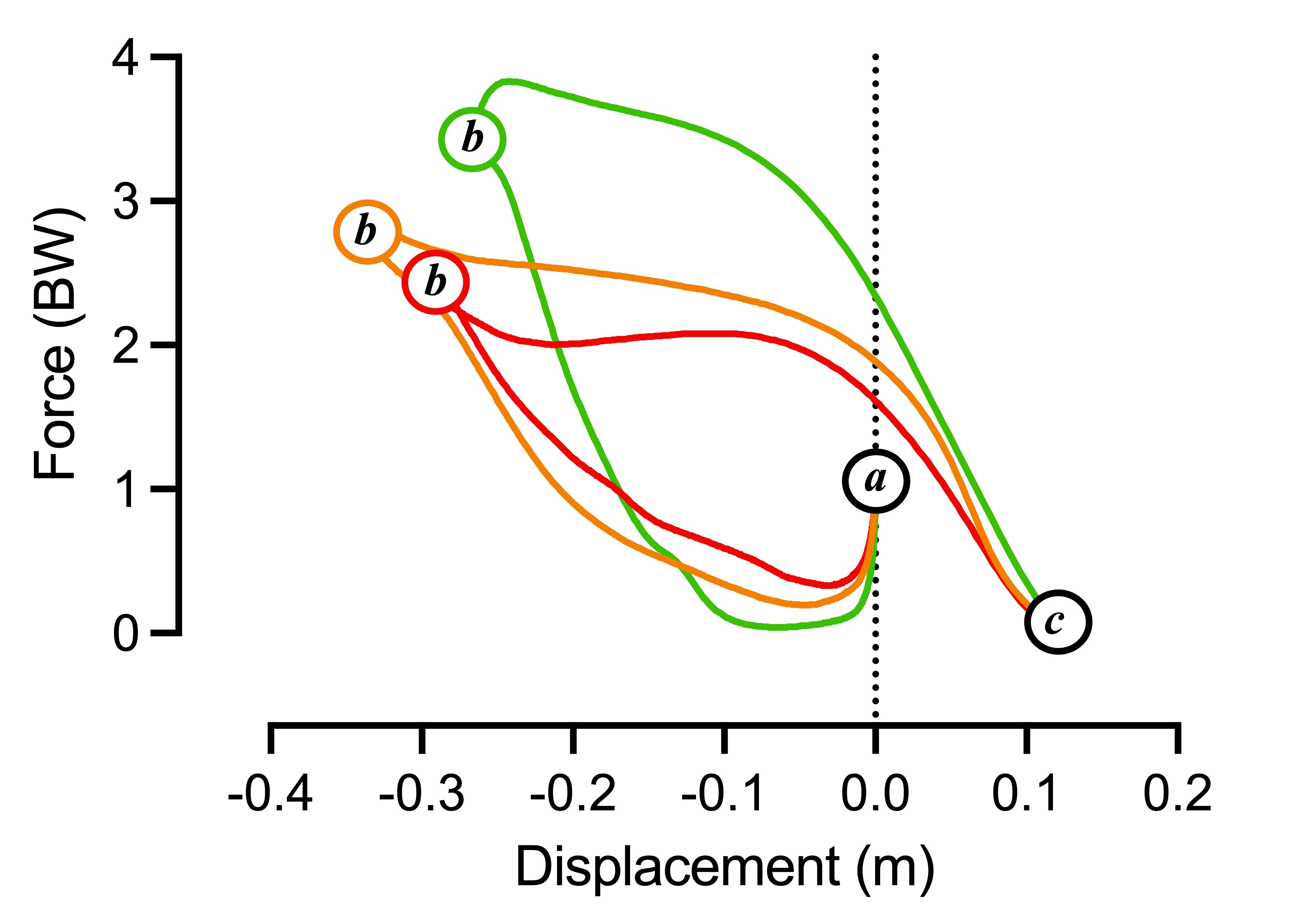
Figure 5: Annotated overlayed colored force-displacement loops from the three jumpers.
(C) Their force-velocity loops
The force-velocity loops from each jumper have been overlayed in Figure 6. Here we can immediately see that there are some significant differences. From left to right:
1. Initially, from 'green' to 'red' jumper, there is a difference between how much the jumpers unweight and how quickly they do this.
2. This difference increases as we move into the braking phase (approximately the second half of the period between points 'a' and 'b').
3. Differences continue to increase and are reflected by differences in the applied force (relative to body weight) and the subsequent movement velocity.
Remember that movement velocity is driven by impulse, where the impulse is the product of how much net force (force less body weight) we can apply and how long we apply it for (see equation below).
F × Δt = m × Δv
In the above equation, F is net force (force less the weight of the jumper and any additional load they're jumping with), t is time, m is the jumper's mass (and any additional load they're jumping with), and v is velocity. For clarity, the triangle symbols are the Greek symbol delta and represent a 'change in'. Clearly, our 'green' jumper applies much more force than either the 'amber' or 'red' jumper and we can see the impact this has had on movement velocity: the impulse-momentum relationship in action (and why I go on about it so much!). For me, the force-velocity loop can really help highlight differences either between the CMJ test results of an athlete over time or between the CMJ test results of different athletes and I think it can make a really impactful addition to the practitioners' athlete assessment toolbox.
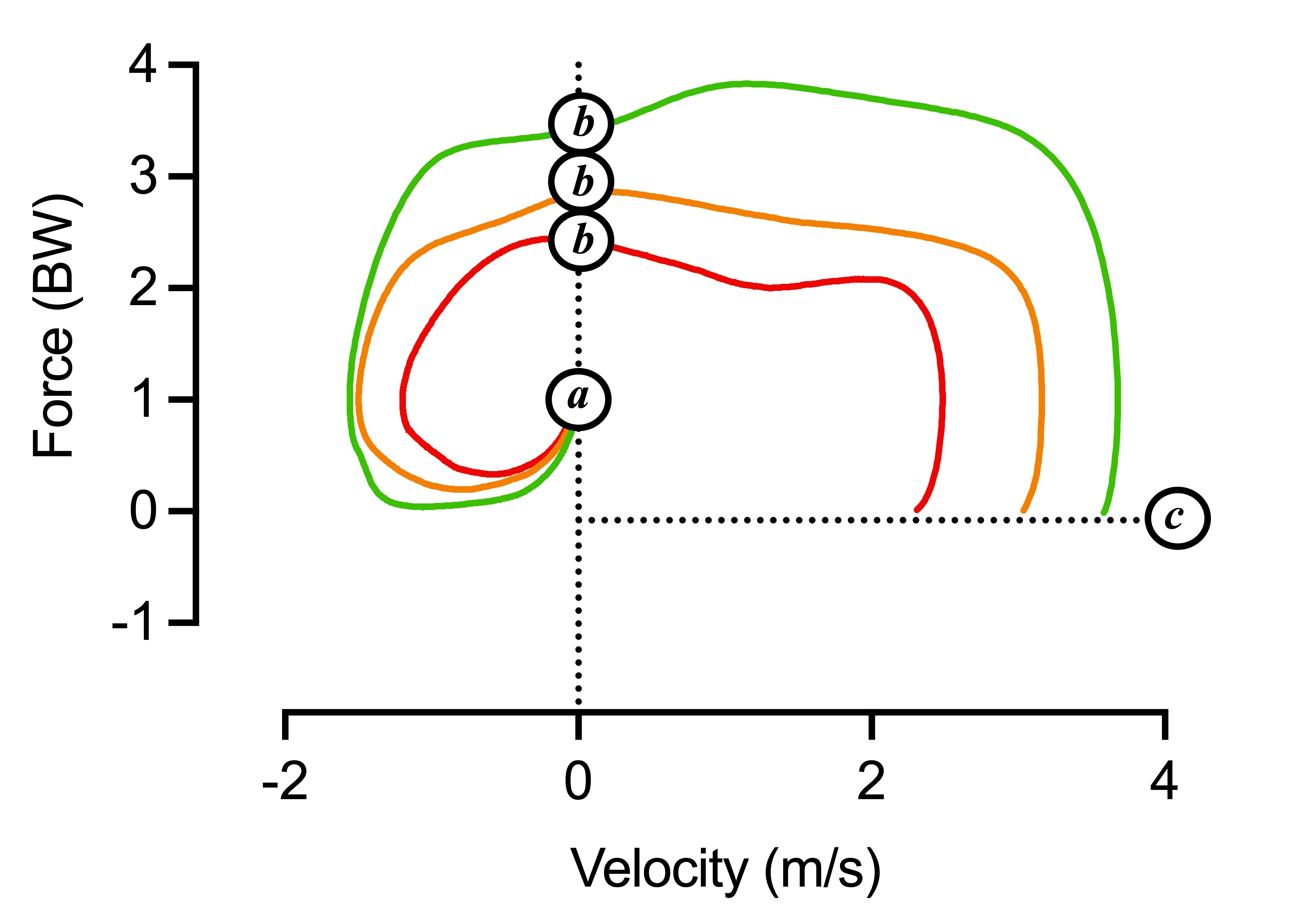
Figure 6: Annotated overlayed colored force-velocity loops from the three jumpers.
Loops in Hawkin Dynamics Software!